HYSPLIT model
The Hybrid Single-Particle Lagrangian Integrated Trajectory (HYPSLIT) model by the National Oceanic and Atmospheric Administration (NOAA) is used to compute simple air parcel trajectories, complex transport, dispersion (e.g., of pollutants and hazardous materials), chemical transformation, and deposition simulations (Air Resources Laboratory, 2020; Stein et al., 2015). The HYSPLIT model has been applied to scenarios such as wildfire smoke events, release and dispersal of radioactive material, and volcanic eruptions. Its calculation method combines Lagrangian and Eulerian approaches; the former uses a moving frame of reference to calculate advection and diffusion when trajectories/air parcels move away from their starting point and for simulating transport, dispersion, and deposition, while the latter works with a 3D grid reference to calculate pollutant air concentrations (Stein et al., 2015).
Scenario: Huge Release of Radioactive Substances in Chernobyl
Since 1977, Chernobyl (formerly under the Soviet Union) had invested in nuclear power to strengthen the Soviet in the Cold War and installed four RMBK reactors that are situated in what is now the border between Ukraine and Belarus (Blakemore, 2019). On April 26, 1986, at around 01:24 local, the workers conducted an experiment to test safety equipment, but violated safety protocols and made a significant error (especially with poor design in the system) that caused explosions (Onishi, Voitsekhovich, and Zheleznyak, 2006). Not long after the first steam explosion, the nuclear plant reactor was then exposed to the oxygen in the air, causing a graphite fire and metals to react with water (which produced hydrogen gas that triggered another explosion). Compared to the Hiroshima nuclear bombing, the Chernobyl nuclear explosion released six times more radionuclides (mostly with short half-lives, from hours to just a few days), but the number of deaths from direct effects is smaller (31 people vs. up to thousands of people in Hiroshima). The contaminated clouds had actually spread throughout the world, not just to parts of Europe (Chernobylwel.come, 2020). Some of the material released have half-lives that outlive many generations, e.g., U-235 with 700 million years (Wendorf, 2019). Thousands of people and wildlife that were particularly in its vicinity have been significantly affected by it—for instance, indirect health effects which increase mortality are still evident to this day. Although the event happened many years ago, it is still relevant as its negative impacts will continue to persist in the future. Concerning climate change, there have been studies recently regarding the explosion’s connection to severe wildfires and drought in the affected regions. With higher tree mortality and lower decomposition rates, there is a larger risk of fueling wildfire events in countries such as Ukraine and Belarus (Evangeliou et al., 2015).
Synoptic Maps
Synoptic maps are helpful in observing certain process relating to e.g., local weather patterns and seasonal differences by understanding the low- and high-pressure systems. Low-pressure systems (cyclonic) are typically associated with cloudy skies and precipitation, and high-pressure systems (anticyclonic) with clear skies. These systems allow us to look at the wind direction that is influenced by the Coriolis effect. For this scenario in the Northern Hemisphere, low-pressure systems have a counter-clockwise motion while high-pressure systems with clockwise motion.
As shown in Figure 1, much of Europe and western Ukraine generally have lower atmospheric pressure at sea level, while western Russia is shown to be in a high-pressure system on April 26. The isobars in the sea level pressure map show that southeasterly winds travel over regions near the border between Ukraine and Russia and up to the north (Scandinavia). Troughs, which are associated with unstable air, wet and colder conditions, seem to occur on the west and south of Ukraine (from 1012 to 1018 hPa, e.g., 30E to 45E). On the other hand, a ridge of high pressure (which is associated with dry and warm conditions) is shown coming from the northeast to Ukraine (from 1030 to 1017 hPa).
Geopotential heights in Figure 2 represent the heights/elevations of surface pressures above sea level. Since cold air is dense, it sinks and pushes the surface pressure height (at 500 hPa) lower; conversely, warm air is less dense and, therefore, increases the 500 hPa surface pressure height. Colder air has more pressure than warmer air; this means that pressure increases with decreasing height.
In Figure 2, we can see that the height precisely on the south of Ukraine is lowest (552 hPa) in that area. As we move further away from that centre, the elevations increase (560-567 hPa). This means that the air temperature from the centre increases with geopotential height. Like in the sea level pressure map, systems of high- and low-pressure can be determined with the geopotential heights. For example, the area where the lower temperatures (lower heights) are found in the centre represents a low-pressure system and in increased heights is a high-pressure system. And above it is the ridge of high pressure over west Russia moving towards the northwest.
The isobars in Figure 1 and the geopotential heights that are close to each other (generally in between the low- and high-pressure systems) denote strong, powerful winds over these levels. In Figure 2, these strong winds can be found at the ridges of high pressure that surround the low-pressure system on Ukraine. The geopotential height map also follows the wind source and direction shown in the mean sea level pressure map.
Trajectory Runs
Several sources have mentioned the height (from 1500m up to 3000m) at which much of Chernobyl debris has been confined in the lower atmosphere. Yet, around a month after the incident, some of the material were found to have reached and entered the lower stratosphere (~10000m) (Kownacka and Jaworowski, 1994). Thus, for the trajectory map, I chose the second and third height to be 2000m and 8000m, respectively.
A backward-trajectory analysis is very common and used to locate where the air particles originate from. However, for this assignment, the forward-trajectory is used to determine where the particles will go from the source, which has been identified for the Chernobyl scenario. At lower heights, 500-2000m, the trajectories suggest that the mass released would have been dispersed towards the north and eventually to the east (towards Russia) over the 72-hr period following the event on April 26. Meanwhile, at heights close to the stratosphere (i.e., 8000m), the trajectory loops around Ukraine and its adjacent countries. The trajectories also resemble the pattern found especially in Figure 2, such as where the 8000m trajectory follows the anti-clockwise wind direction of the low-pressure system that sits mostly in Ukraine.
Concentration Run
Due to political conflicts, the Soviet initially attempted to deny the accident. The radioactive material from the explosion reached to about a height of 1500m, at which southeastern wind carried the radioactive cloud towards the countries in the north (Chernobylwel.come, 2020)—as seen in the forward trajectory and dispersion maps.
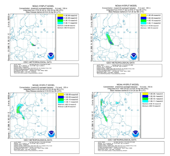
Furthermore, both sea level pressure and geopotential height maps, again, can help explain the direction of the strong winds responsible for the initial transport of pollutants from Chernobyl to Scandinavia. Larger concentrations in dark blue are shown to have lasted at least 24 hours since the explosion (April 26-27, Figure 1). On April 28, the concentration has started to disperse and move eastward to other parts of Scandinavia, and by April 29, smaller concentrations move further to Russia.
The Role of Synoptic Meteorology, Limitations of the HYPSLIT model
As what we see on the maps, synoptic meteorology helps us determine the source or trajectories of pollutant(s), and the relative levels of concentrations over a given area. Several factors like solar radiation, precipitation, mixing depths, air temperatures, and wind speeds can affect air pollution. With stronger winds blowing from the southeast (represented as isobars/geopotential heights in between high and low-pressure systems), the elevated concentrations of released radioactive materials from Chernobyl are being pushed and dispersed further towards the northwest, eventually decreasing pollutant concentrations over the northern regions. Rainfall can decrease air pollution as well by washing away particulate matter and soluble pollutants (The National Weather Service, n.d.); the low-pressure system near Scandinavia could have possibly decreased the concentrations coming from Chernobyl, if these regions had rainfall at that period.
The trajectory and concentration runs generally agree with the patterns shown in the synoptic maps. However, the synoptic maps only show the values for one day (April 26), while the other maps are a dynamic representation of the release within longer durations, i.e., 72 hours. Therefore, the isobars and geopotential heights in the synoptic maps do not necessarily shape how the trajectories will appear. In addition, the trajectories also can also show different patterns from those in the sea level pressure map when looking at higher altitudes above sea level.
The HYPSLIT modelling has limitations, as outlined by NOAA, that ignores some important effects, such as those of the chemistry of the pollutants and gases, varying emission rates from sources other than volcanoes, or complex terrain, that can change the trajectories. For example, the model does not consider how the Alps mountain range in Europe may influence the trajectories of the pollutants.
References
Air Resources Laboratory. (2020). NOAA: Air Resources Laboratory. Retrieved from HYSPLIT-2-Air Resources Laboratory: https://www.arl.noaa.gov/hysplit/hysplit/
Blakemore, E. (2019, May 17). The Chernobyl disaster: What happened, and the long-term impacts. Retrieved from National Geographic: https://www.nationalgeographic.com/culture/topics/reference/chernobyl-disaster/
CHERNOBYLwel.come. (2020). CHERNOBYL HISTORY. Retrieved from CHERNOBYLWEL.COMe: https://www.chernobylwel.com/chernobyl-history
Evangeliou, N., Balkanski, Y., Cozic, A., Hao, W. M., Mouillot, F., Thonicke, K., . . . Møller, A. P. (2015). Fire evolution in the radioactive forests of Ukraine and Belarus: future risks for the population and the environment. Ecological Monographs, 85(1), 49-72. Retrieved November 1, 2020, from http://www.jstor.org/stable/24818231
Kownacka, L., & Jaworowski, Z. (1994, November). Nuclear weapon and Chernobyl debris in the troposhere and lower stratosphere. The Science of the Total Environment, 144(1-3), 201-215. Retrieved from https://doi.org/10.1016/0048-9697(94)90439-1
Onishi, Y., Voitsekhovich, O. V., & Zheleznyak, M. J. (2006). Chernobyl - what have we learned? : The successes and failures to mitigate water contamination over 20 years. Springer.
Stein, A. F., Draxler, R. R., Rolph, G. D., Stunder, B. J., Cohen, M. D., & Ngan, F. (2015). NOAA's HYSPLIT Atmospheric Transport and Dispersion Modelling System. Bulletin of the American Meteorological Society, 96(12), 2059-2077. doi:10.1175/bams-d-14-00110.1
The National Weather Service. (n.d.). Clearing the Air on Weather and Air Quality. Retrieved from National Weather Service: National Oceanic and Atmospheric Administration: https://www.weather.gov/wrn/summer-article-clearing-the-air
Wendorf, M. (2019, May 11). Chernobyl - A Timeline of The Worst Nuclear Accident in History. Retrieved from Interesting Engineering: https://interestingengineering.com/chernobyl-a-timeline-of-the-worst-nuclear-accident-in-history